splot.esda.plot_moran_bv

splot.esda.plot_moran_bv(moran_bv, aspect_equal=True, scatter_kwds=None, fitline_kwds=None, **kwargs)

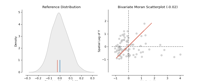
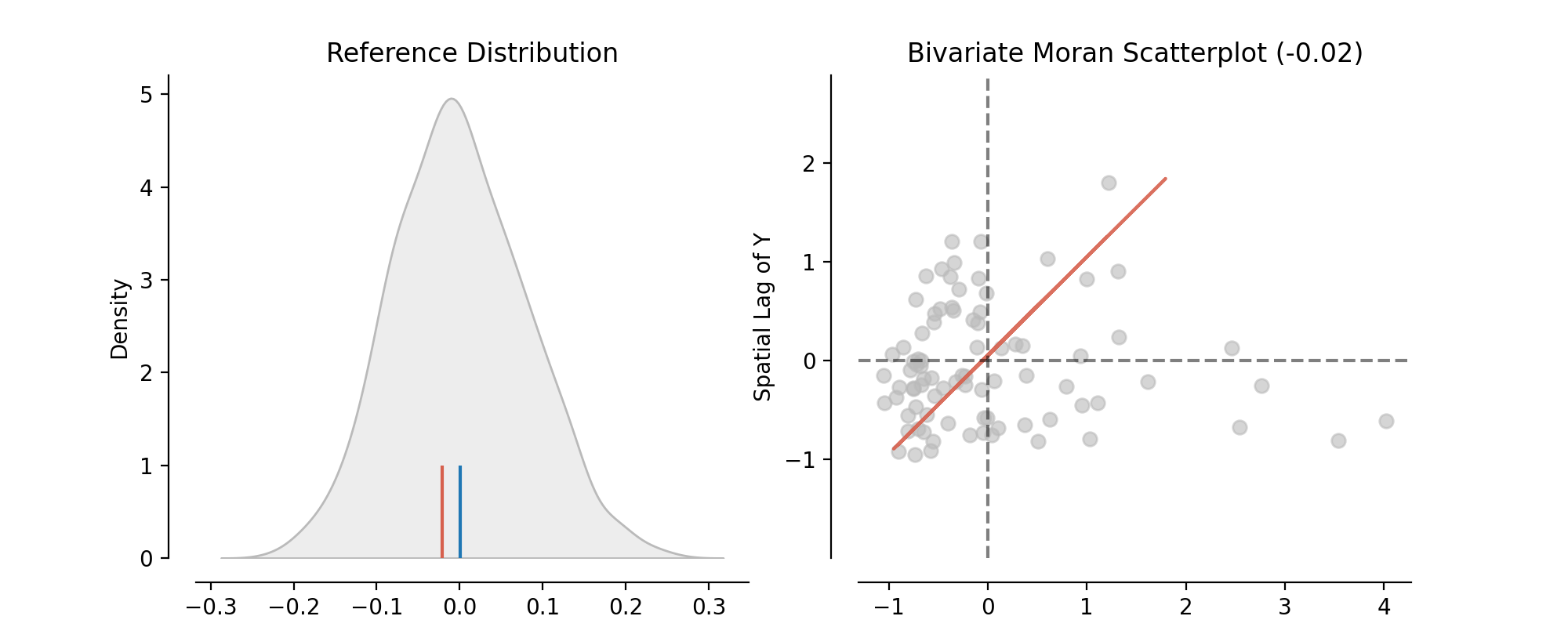
Bivariate Moran’s I simulated reference distribution and scatterplot.

Parameters

moran_bvesda.moran.Moran_BV instance

Values of Bivariate Moran’s I Autocorrelation Statistics

aspect_equalbool, optional

If True, Axes of Moran Scatterplot will show the same aspect or visual proportions.

scatter_kwdskeyword arguments, optional

Keywords used for creating and designing the scatter points. Default =None.

fitline_kwdskeyword arguments, optional

Keywords used for creating and designing the moran fitline and vertical fitline. Default =None.

**kwargskeyword arguments, optional

Keywords used for creating and designing the figure, passed to seaborne.kdeplot.

Returns

figMatplotlib Figure instance

Bivariate moran scatterplot and reference distribution figure

axmatplotlib Axes instance

Axes in which the figure is plotted

Examples

Imports

>>> import matplotlib.pyplot as plt
>>> from libpysal.weights.contiguity import Queen
>>> from libpysal import examples
>>> import geopandas as gpd
>>> from esda.moran import Moran_BV
>>> from splot.esda import plot_moran_bv

Load data and calculate weights

>>> guerry = examples.load_example('Guerry')
>>> link_to_data = guerry.get_path('guerry.shp')
>>> gdf = gpd.read_file(link_to_data)
>>> x = gdf['Suicids'].values
>>> y = gdf['Donatns'].values
>>> w = Queen.from_dataframe(gdf)
>>> w.transform = 'r'

Calculate Bivariate Moran

>>> moran_bv = Moran_BV(x, y, w)

plot

>>> plot_moran_bv(moran_bv)
>>> plt.show()

(Source code, png, hires.png, pdf)

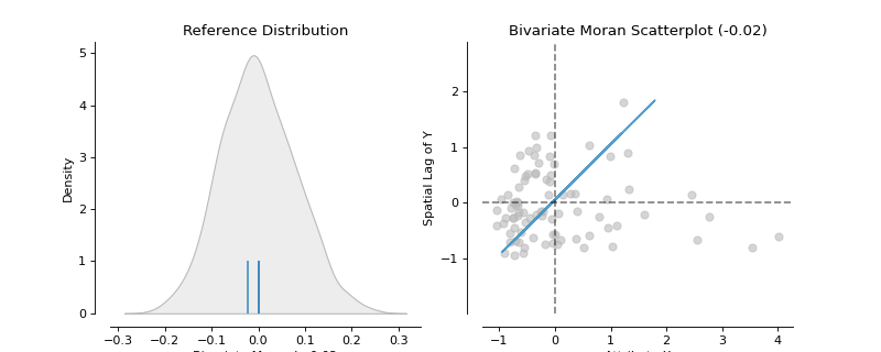
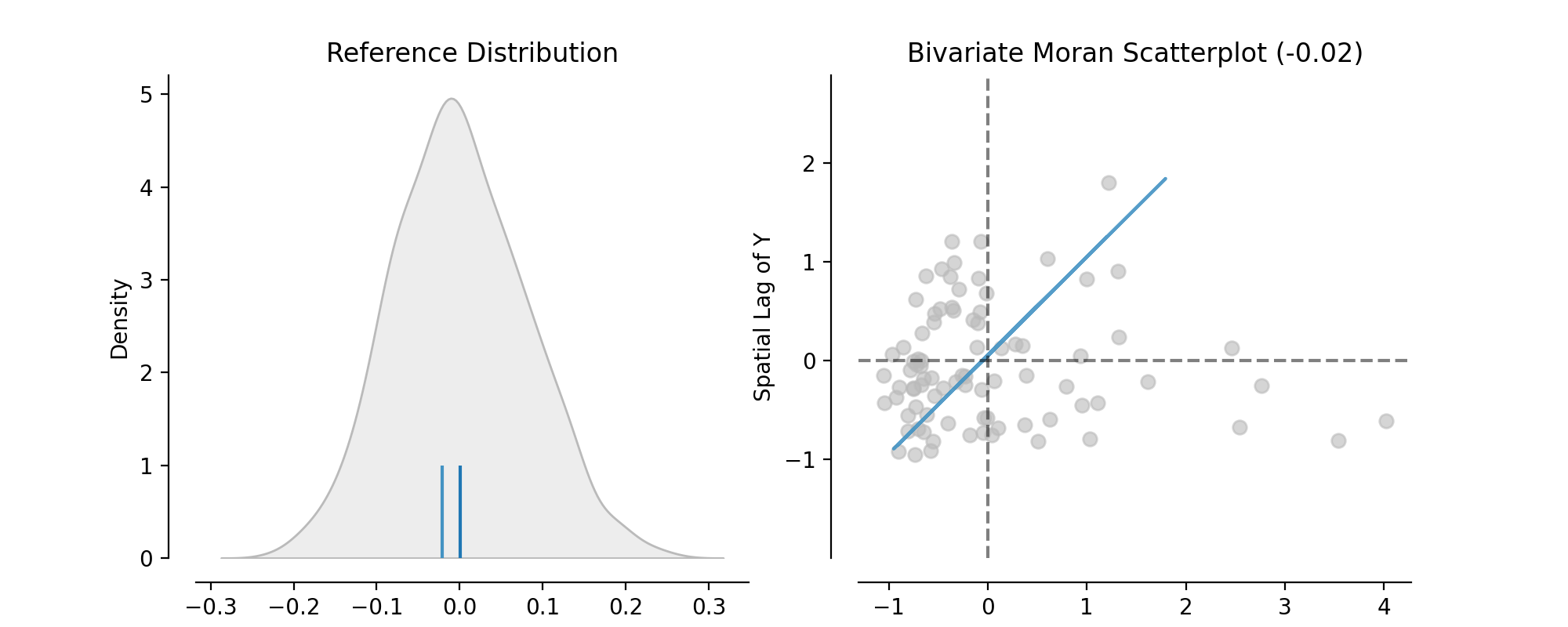
customize plot

>>> plot_moran_bv(moran_bv, fitline_kwds=dict(color='#4393c3'))
>>> plt.show()

(png, hires.png, pdf)