splot.esda.lisa_cluster
- splot.esda.lisa_cluster(moran_loc, gdf, p=0.05, ax=None, legend=True, legend_kwds=None, **kwargs)[source]
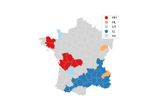
Create a LISA Cluster map
- Parameters
- moran_locesda.moran.Moran_Local or Moran_Local_BV instance
Values of Moran’s Local Autocorrelation Statistic
- gdfgeopandas dataframe instance
The Dataframe containing information to plot. Note that gdf will be modified, so calling functions should use a copy of the user provided gdf. (either using gdf.assign() or gdf.copy())
- pfloat, optional
The p-value threshold for significance. Points will be colored by significance.
- axmatplotlib Axes instance, optional
Axes in which to plot the figure in multiple Axes layout. Default = None
- legendboolean, optional
If True, legend for maps will be depicted. Default = True
- legend_kwdsdict, optional
Dictionary to control legend formatting options. Example:
legend_kwds={'loc': 'upper left', 'bbox_to_anchor': (0.92, 1.05)}Default = None- **kwargskeyword arguments, optional
Keywords designing and passed to geopandas.GeoDataFrame.plot().
- Returns
- figmatplotlip Figure instance
Figure of LISA cluster map
- axmatplotlib Axes instance
Axes in which the figure is plotted
Examples
Imports
>>> import matplotlib.pyplot as plt
>>> from libpysal.weights.contiguity import Queen
>>> from libpysal import examples
>>> import geopandas as gpd
>>> from esda.moran import Moran_Local
>>> from splot.esda import lisa_cluster
Data preparation and statistical analysis
>>> guerry = examples.load_example('Guerry')
>>> link_to_data = guerry.get_path('guerry.shp')
>>> gdf = gpd.read_file(link_to_data)
>>> y = gdf['Donatns'].values
>>> w = Queen.from_dataframe(gdf)
>>> w.transform = 'r'
>>> moran_loc = Moran_Local(y, w)
Plotting
>>> fig = lisa_cluster(moran_loc, gdf)
>>> plt.show()
(Source code, png, hires.png, pdf)